locomotion-classification.github.io
Locomotion Mode Classification based on Wearable Sensor data from Lower Limb Biomechanics
1 Introduction
Characterization of human movement and understanding of corresponding muscle coordination over various locomotion modes and terrain conditions are crucial for determining human movement strategies in environments more prevalent to community ambulation. Biomechanical data captured during locomotion, such as, Electromyography (EMG) signals, can be used to anticipate transitions from one mode to another. Moreover, combination of multiple sensor data has the possibility to assist in data-driven model development for locomotion intent recognition using Machine Learning (ML) to greatly accelerate such tasks.
2 Problem Definition
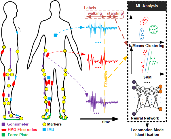
In this project, we propose to combine multiple 3-dimensional biomechanical and wearable sensor data (EMG, Goniometer (GON), Inertial Measurement Unit (IMU) etc.) along with gait information to classify locomotion modes (e.g. idle position, standing position, level-ground walking, stair-ascent, stair-descent, ramp-ascent and ramp-descent) from a single time-sample (hence instantaneous) which might be helpful in predicting a person’s ongoing locomotion mode and develop assistive devices in future.
We will develop subject-dependent classification models for 7 possible modes (idle, standing and 5 movements) regardless of their terrain conditions based on biomechanics data captured from lower limbs of able-bodied participants using EMG, GON, IMU etc. sensors. Details of chosen sensors and classification labels are provided in Section 4.2.
3 Literature Review
The study in [1] focused only on linear relationships between variables and terrain conditions. In this work, we will explore possible higher order relationships and develop ML models to classify locomotion modes. As the dataset has been released only recently(Feb. 2021), this will be one of the first studies on this dataset along this direction. Recently, gait phase estimation during multimodal locomotion from just IMU data [2], and subject-independent slope prediction from just IMU and biomechanical data [3] using Convolutional Neural Network have been reported for exoskeleton assistance. However, in this study, we will combine data from multiple wearable sensors, thus providing a more comprehensive picture.
4 Data Collection
4.1 Finding Data
The public dataset acquired by EPIC Lab at Georgia Tech has been adopted for the current project.
The dataset contains 3-dimensional biomechanical and wearable sensor data (EMG - 11 muscles, Goniometer (GON) - 3 body parts, Inertial Measurement Unit (IMU) - 4 body parts) along with the kinematic and kinetic profiles of joint biomechanics (as a function of gait phase) from right side of the body of 22 young and able-bodied adults for various locomotion modes (e.g. level-ground or treadmill walking, stair-ascent, stair-descent, ramp-ascent and ramp-descent), multiple terrain conditions for each mode (walking speed, stair height, and ramp inclination) and multiple trials [1]. The following figure shows the different sensor placements in that study[1]:
In this project, we will work on a randomly chosen subset of the data, i.e., we focus on sensor data collected from a single participant (e.g. AB21) and consider all possible terrain conditions and selected locomotion modes and related sensors.
4.2 Cleaning and Merging Data
The dataset has an organized directory structure containing timestamps and corresponding locomotion labels. During data exploration, we have excluded Treadmill terrain condition from our considered dataset, as it does not contain the corresponding labels. It, however, contains walking/running speeds, which can be a regression analysis task, based on the sensor data, and as such, was not considered in this study. Henceforth, we consider these three terrain conditions: Levelground, Ramp, and Stair.
Some of the biomechanics data had missing data values (NaN or Not-a-Number) or low information content, such as ‘Inverse Kinematics’ (ik), ‘Inverse Dynamics’ (id), ‘Joint Power’ (jp), and ‘Force Plate’ (fp). We have not considered them as well. In particular, we focused on the following 5 sensors:
gon: Goniometer data from hip, knee, and ankle, sampled at 1000 Hz. These sensors contribute 5 raw features, based on their placements around the body:ankle-sagittal, ankle-frontal, knee-sagittal, hip-sagittal and hip-frontal.emg: Electromyography data from 11 muscles, sampled at 1000 Hz. Accordingly, these sensors contribute 11 raw features:gastrocmed, tibialisanteriror, soleus, vastusmedialis, vastuslateralis, rectusfemoris, bicepsfemoris, semitendinosus, gracilis, gluteusmedius, rightexternaloblique.gcLeft: Gait cycle segmented by heel strike or toe off of left foot, sampled at 200 Hz. These contribute 2 raw features:HeelStrike and ToeOff.gcRight: Gait cycle segmented by heel strike or toe off of right foot, sampled at 200 Hz. These contribute 2 raw features:HeelStrike and ToeOff.imu: Inertial Measurement Unit data from trunk, thigh, shank, and foot segments, sampled at 200 Hz. These contribute 24 raw features:foot-Accel_X, foot-Accel_Y, foot-Accel_Z, foot-Gyro_X, foot-Gyro_Y, foot-Gyro_Z, shank-Accel_X, shank-Accel_Y, shank-Accel_Z, shank-Gyro_X, shank-Gyro_Y, shank-Gyro_Z, thigh-Accel_X, thigh-Accel_Y, thigh-Accel_Z, thigh-Gyro_X, thigh-Gyro_Y, thigh-Gyro_Z, trunk-Accel_X, trunk-Accel_Y, trunk-Accel_Z, trunk-Gyro_X, trunk-Gyro_Y, trunk-Gyro_Z
Moreover, in this study, we consider only 7 locomotion modes, specifically, idle, walk, stand, stair-ascent, stair-descent, ramp-ascent, and ramp-descent. Consequently, the problem becomes that of a classification task with 7 output classes and 44 (= 5+11+2+2+24) input features.
Data merging process involved concatenating data from different locomotion modes, different sensors, and different acquisition campaigns. As you might notice, the sensor data are sampled at two different sampling frequencies (200 Hz and 1000 Hz). We chose to downsample the high frequency data to align the features. Also, we had to get rid of the time samples that contain sensor data for locomotion modes, such as, ‘stand-walk’, ‘walk-stand’ or ‘turn’, as we do not consider them in this study.
As a result of the choices made in the above and data cleaning, we end up with 256,085 data samples, each containing 44 features for one of the 7 class labels. For supervised classification tasks, we have used 80% of the total data (204,868 samples) for training and validation (80% for training, 20% for validation), and kept aside 20% (51,217 samples) as test data. For methods where a validation set is not required, we use both the training and validation sets to build the models.
4.3 Data Pre-Processing
4.3.1 Signal Conditioning
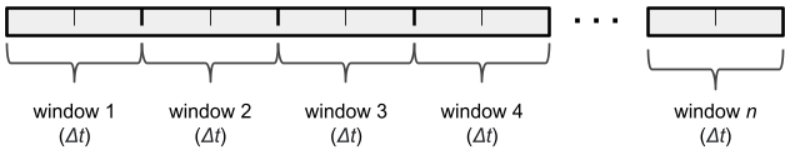
Although the data has been appropriately filtered for the specific sensors, we may have to further pre-process the raw data (e.g. rectification and low-pass filtering of EMG data) due to possibly unaccounted-for factors such as skin conditions, electrode placements, and anatomical differences between the subjects. The original dataset consists of several features representing individual sensor channels. Each feature is sampled at a rate of 200 Hz, resulting in a large number of samples. However, for noisy data, especially EMG data, this data can be difficult to classify without processing (which will be evident from the results presented in the following). One method of doing so is to collect samples in a moving window of time, and create features for each window of time [4]. For this project, each window occurs in series after the previous one, as seen in the figure below, with gaps occurring whenever there are breaks in the time series data.
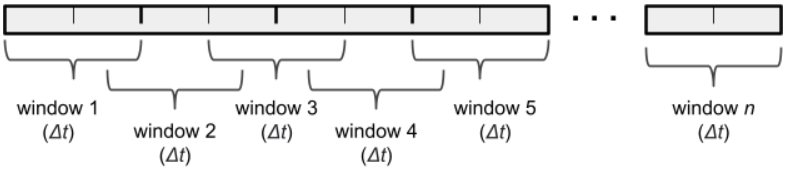
For each time window, 5 sub-features were extracted from each feature: the maximum and minimum values in that window, the mean value of the window, the standard deviation of values in that window, and the final value in the window. The mean and standard deviation were both suggested as good features for use on EMG data [4], while the maximum, minimum, and final data points for each window provide general information about the data in that time interval. These sub-features effectively multiply the number of dimensions of the dataset by 5. While this means that dimensionality reduction will be more intensive, the processed features will end up more informative than the raw data. However, a preliminary study on the aforementioned processed features did not result in improved accuracy. In a future work, we will look at implementing other features than the 5 used here, such as root mean square (RMS) or autoregressive coefficients for EMG data. We also plan to compare the results of using separate windows in sequence with using overlapping windows, as shown in the figure below:
.
4.3.2 Feature Engineering
4.3.2.1 Minimum Redundancy Maximum Relevance (MRMR) Scoring
MRMR Scoring [6] computes pairwise mutual information of features and mutual information a feature and corresponding label to find an optimal set of features that is mutually and maximally different and can represent the class labels efficiently. The algorithm minimizes the redundancy of a feature set and maximizes the relevance of it to the class labels. All of raw data and labels go into the algorithm which scores the features based on their relevance to class labels. In the following, you can see the scores returned by MRMR algorithm for raw sensor data:

As you can see, feature no. 2 (Goniometer, ankle-frontal) has been ranked the highest by the algorithm due to its importance as a predictor for class labels. The others just from raw data seem to be insignificant. This will later be verified by other algorithms later on, and as we will use pre-processing on raw data for the later part of the project, we expect to see improvements in the scores for features from other sensors.
5 Methods
In this project, we will use the aforementioned sensor and biomechanical data as input features and corresponding locomotion modes as classification labels to develop supervised and unsupervised ML models such as k-Means Clustering, Principal Component Analysis (PCA), Linear Discriminant Analysis (LDA), Support Vector Machines (SVM), Random Forest (RF), Decision Trees (DT), and Neural Networks (NN).
5.1 Unsupervised Learning Component
While working on raw data, considering samples from each time point can be insufficient. So, we have looked into two Unsupervised learning algorithms so far, specifically, Principal Component Analysis (PCA) and k-Means Clustering to see if we can reduce the number of dimensions and get better classification results. The results for these methods are reported in Section 6.1.
5.2 Supervised Learning Component
We have employed several Supervised learning algorithms to perform classification task mentioned above, in particular, Linear Discriminant Analysis (LDA), Decision Tree (DT), Support Vector Machine (SVM), Random Forest (RF), Multi-Layer Perceptron (MLP), and Convolutional Neural Network (CNN). The results for these methods are reported in Section 6.2. Note that, although MRMR is a supervised feature ranking algorithm, we have put it under feature engineering as it does not act as a method for classification.
6 Results and Discussion
6.1 Unsupervised Learning Methods
6.1.1 PCA
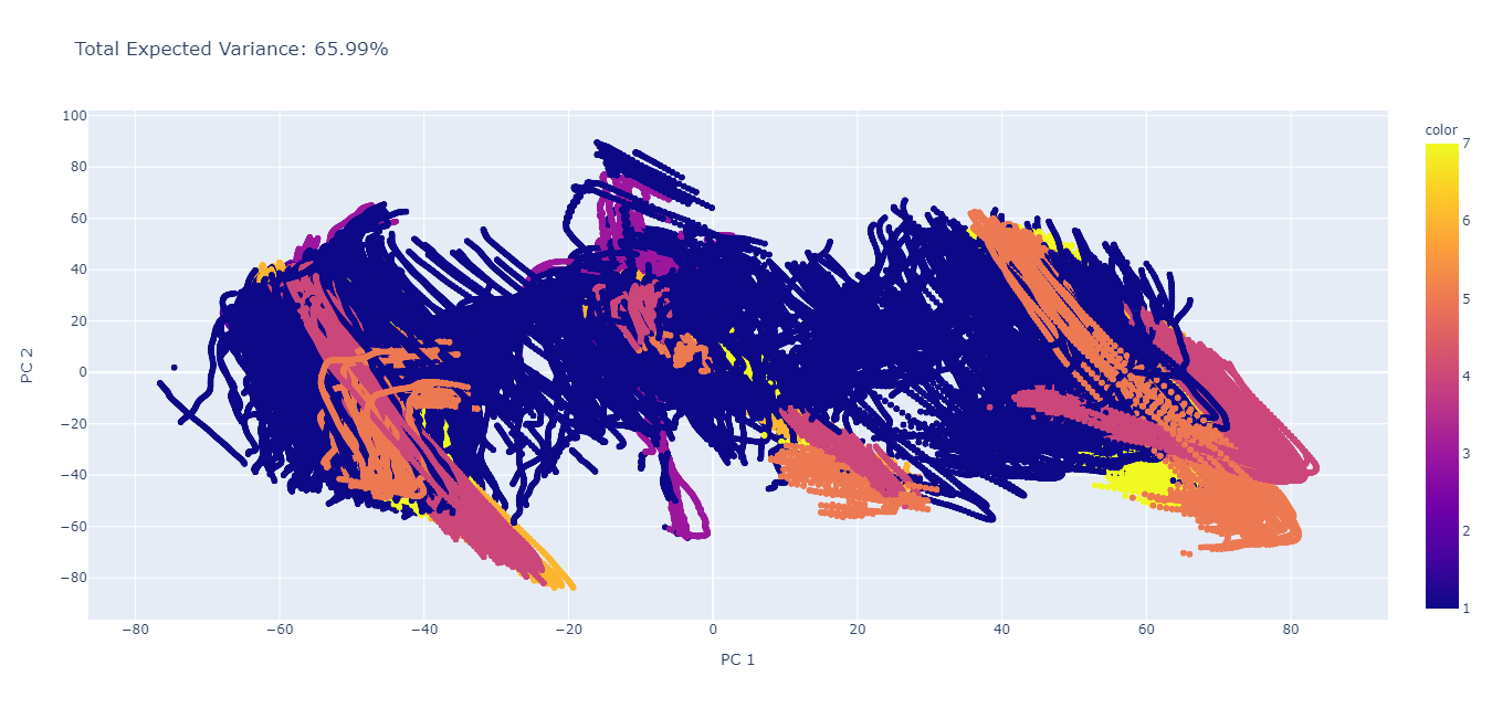
Principal component analysis (PCA), which is a broadly used unsupervised learning algorithm, was performed on the processed data to project it to a lower dimensional space. In essence, PCA was used as a dimensionality reduction algorithm to identify the principal components of our processed data. After performing the PCA, we first analyzed the first two principal components of the analysis (n_components = 2); essentially, this is looking at reducing the dataset of 44 features to only 2, and analyzing the explained variance captured by the first 2 principal components.
The visualized result as well as the total explained variance for this (PC 1 vs PC 2) is shown in the figure below. Here, we see that the total explained variance is 65.99%, which suggests that using only 2 of the principal components will capture approximately 66% of the variance. In addition, we see that PC1 and PC2 are unable to clearly separate each of the different locomotion labels (labels 1 through 7; 1 - idle, 2 - walk, 3 - stand, 4 - stair ascent, 5 - stair descent, 6 - ramp ascent, 7 - ramp descent).
Thus, we decided to look at additional components to see how much variance is captured with each of the components. Comparisons between the first 10 PCs are shown in the figure below. As seen, when comparing the 8th PC to each of the other PCs, there seems to be a pretty definite separation between each of the different labels. We also see that using 10 PCs describes approximately 99.70% of the variance in the data set (total explained variance is equal to 99.70%).
.png)
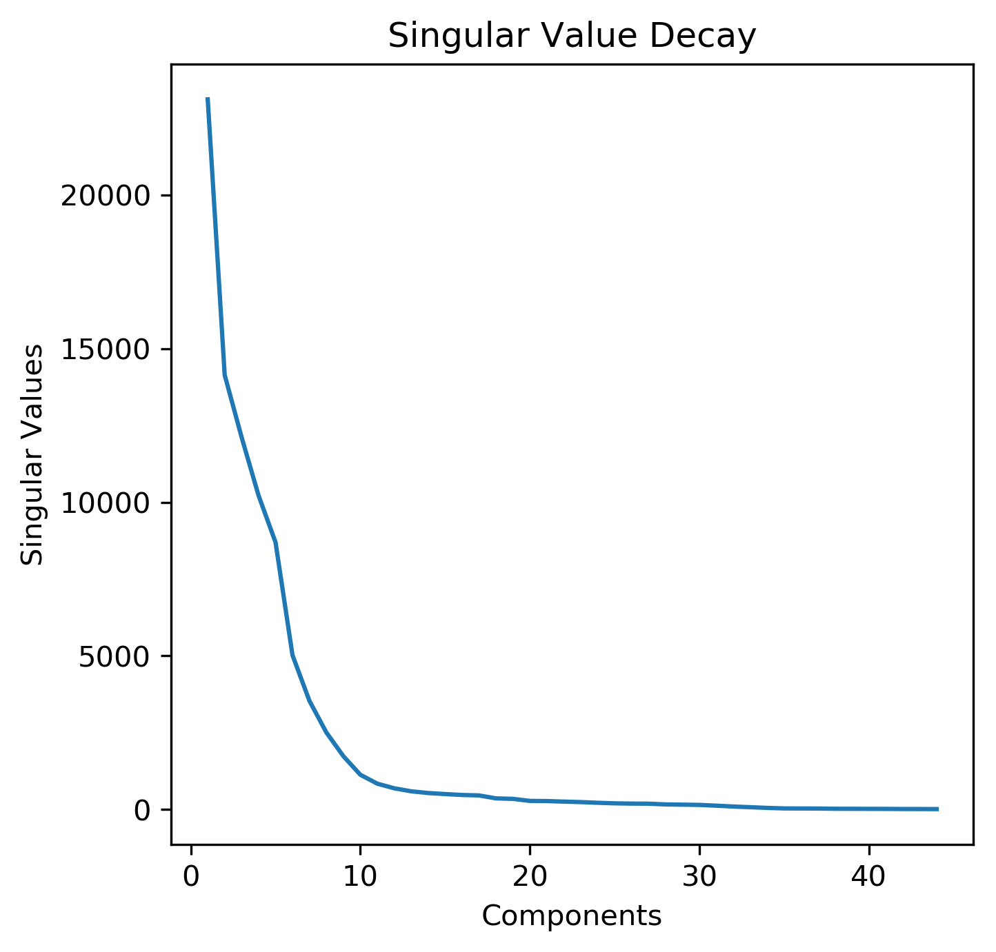
To better understand how many of the principal components should be used in further analysis, we extracted the singular values that are obtained from the Singular Value Decomposition (SVD) when the PCA algorithm is performed. Similar to the Elbow Method utilized in finding the optimum number of clusters for a KMeans analysis, a sharp decline in the singular values would suggest that the entire data set can be appropriately captured by only a few components, which specifically are the eigenvectors associated with the highest singular values. A plot of the captured singular values is shown below. From this, we can see that there is a sharp decline in the singular values following 10 components, which suggests using the first 10 principal components would be sufficient for approximating the entire dataset; these results confirm the previous analysis of the different principal components.
6.1.2 k-Means Clustering
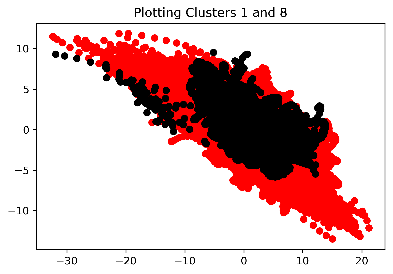
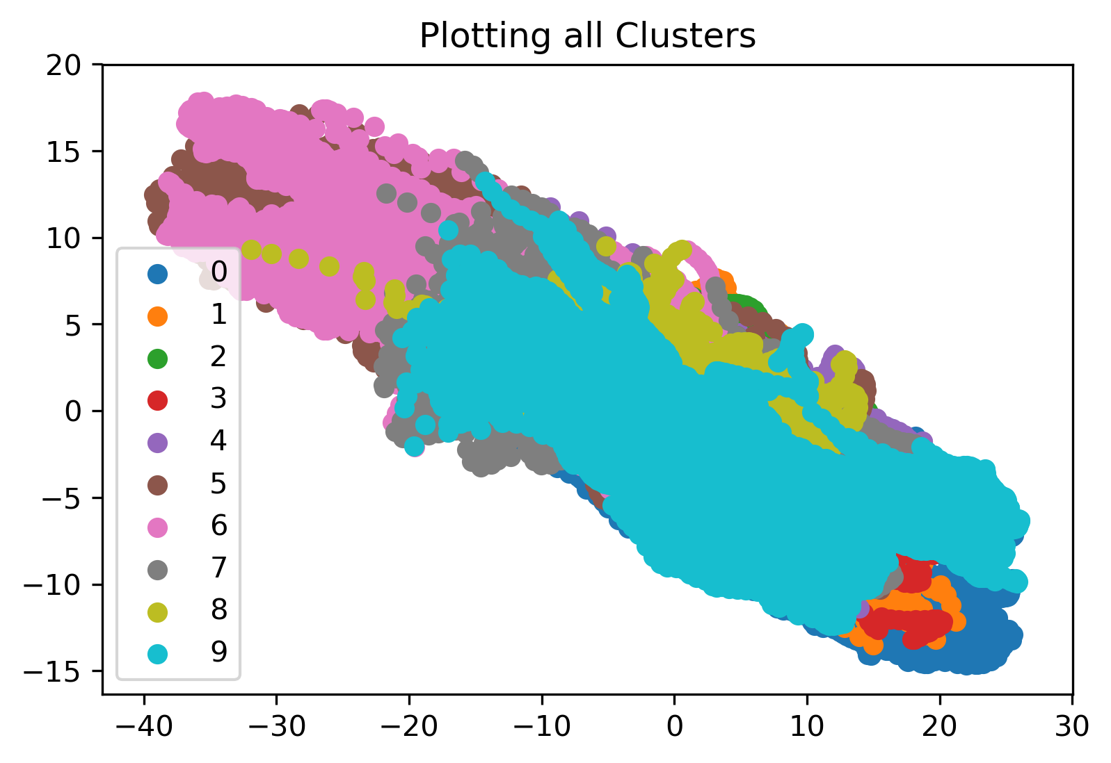
KMeans clustering was employed to compare and contrast all datapoints in our cleaned dataset. We begin by performing the KMeans clustering on the entire dataset as a whole. We initialized the algorithm with 10 clusters to see how the algorithm would cluster all the data points and if there were any interesting takeaways. Results for the first cluster, a comparison of the 2nd and 8th cluster, and a plot displaying all of the labeled clusters are shown in the figures below. From the last plot specifically, we see that all of the clusters are overlapping, which indicates that KMeans may not provide any discernible results.

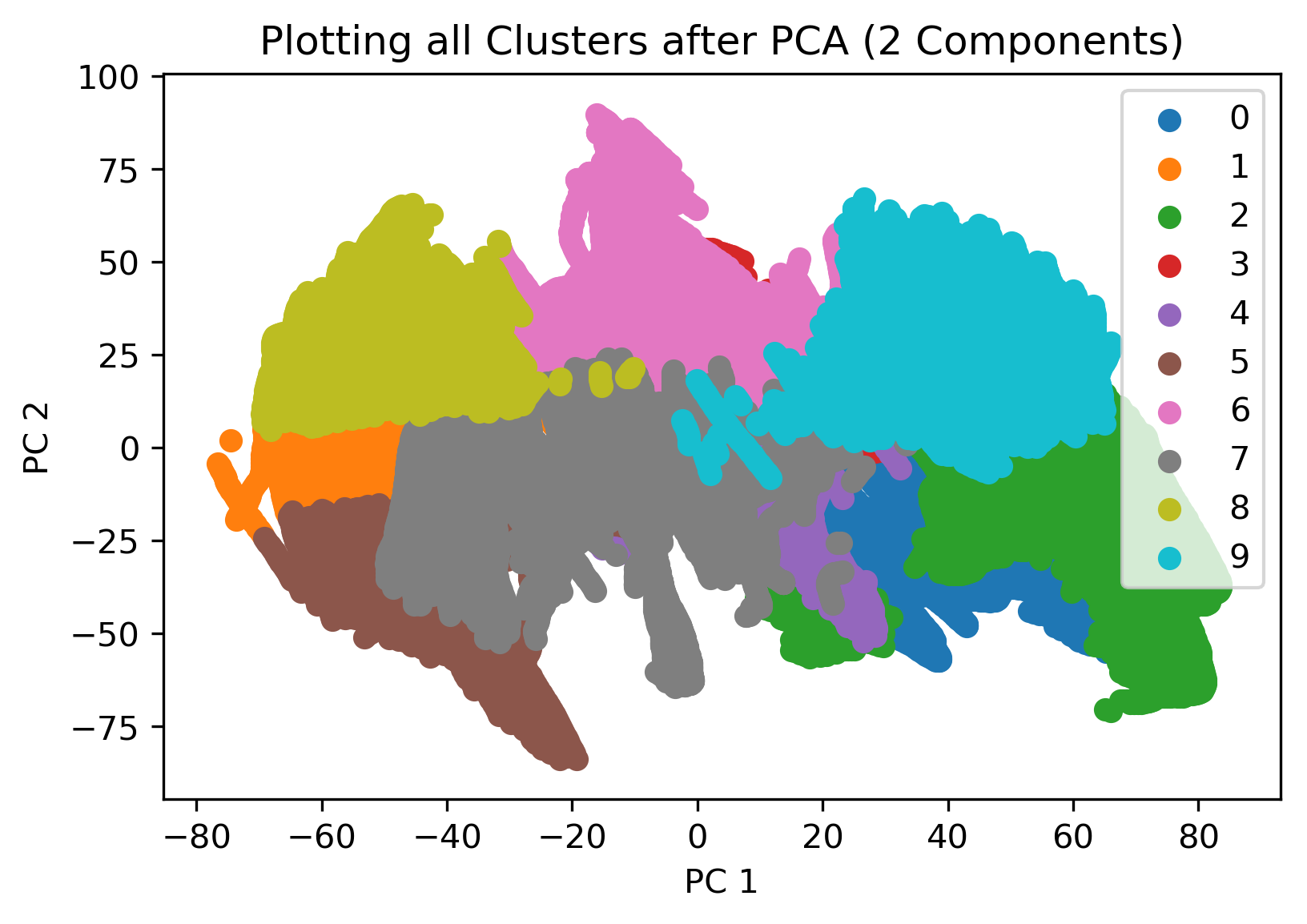
KMeans clustering was also employed after a dimensionality reduction using PCA. Specifically, the data was reduced to the first two principal components (where 66% of the variance is captured, as mentioned previously). In this case again, the number of clusters was defined as 10, and the resulting visualization is shown in the figure below. In this case, we see that after dimensionality reduction, the data has been defined into distinct clusters with no overlap between each.
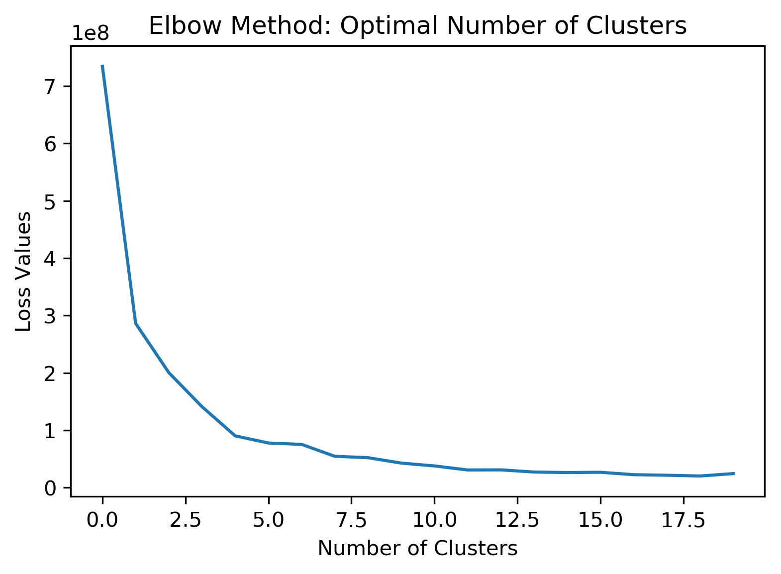
Finally, we perform an elbow method analysis of the data (following PCA/dimensionality reduction) to analyze what the optimal number of clusters would be. Here, the find_optimal_num_clusters function implemented in Homework 2 was applied, and the resulting figure is shown below. Using the elbow method, we see that the optimal number of clusters would be approximately 3 to 4. The number clusters chosen for the initial analysis (10) was greater than the value found using the elbow method.
6.2 Supervised Learning Methods
6.2.1 Naive Bayes Classification
Naive Bayes classification is the application of Bayes theorem with the assumption that there is conditional independence between every pair of features in a given dataset. In this case, we utilize Gaussian Naive Bayes algorithm for classification, which assumes that the likelihood function of the features is Gaussian, as described below; here, the two parameters σ and μ are optimized using the maximum likelihood estimation approach.

The processed dataset is split into training and testing data. The size of the test data is defined to 25% of the processed data set, or 64022 points. After performing Gaussian Naive Bayes classification, the number of mislabeled points out of a total of 64022 points was 22459, which results in a test accuracy of 64.92%. Although this test accuracy may seem low, in relation to our processed dataset it is not too surprising. This is because Gaussian Naive Bayes assumes that the relationship between each of the features is Gaussian in general; however, for our processed dataset, we do not actually know the probabilistic relationship between each of our features and in general they may not be Gaussian (which seems to be the indicataion from the resulting test accuracy).
6.2.2 LDA
In Discriminant Analysis, it is assumed that each class generates features using a multivariate normal distribution, i.e., the model assumes that the data samples have a Gaussian mixture distribution. In Linear Discriminant analysis, the model has the same covariance matrix for each class, with different means. It predicts in a way that minimizes the classification cost defined by posterior probability of classes and cost of misclassification. LDA achieves 68.41% test accuracy on raw data, compared to 14.2% which would be for random class assignments, and thus contains significant results on just raw data.
After performing PCA, LDA achieves 68.41% test accuracy with no dimensionality reduction, so, PCA without pruning does not improve accuracy for LDA. Further study needs to be done on LDA after PCA-based dimensionality reduction.
6.2.3 DT
Binary Decision Tree for multiclass classification has been fitted to the training data based on the features and class labels. The binary tree creates node splitting for the feature vectors based on impurity or node error. Curvature Test (a statistical test assessing the null hypothesis that two features are unassociated) was chosen so that the decision tree classifier chooses the split predictor that minimizes the p-value of chi-square tests of independence between each feature and the class label [5]. The fitted decision tree achieves 96.81% test accuracy. Also, an estimation of predictor importance values can be computed by summing changes in the risk due to splits on every feature and dividing the sum by the number of branch nodes, which results in the following graph.

As we can see, Goniometer sensor data have been ranked the highest as features using Decision Tree based analysis as well.
In the following, we report relevant ML_metrics evaluation for Decision Tree Classifier, which we will later extend to the other classification algorithms.
| Scoring Metric | Performance Value |
|---|---|
| accuracy | 96.75% |
| balanced_accuracy_score | 96.93% |
| precision_score_macro | 0.9678 |
| recall_score_macro | 0.9693 |
| f1_score_macro | 0.9685 |
We also report the confusion matrix for this classifier:
6.2.4 SVM
SVM classifier has been trained with Radial Basis Function kernel. An exploration of different kernel methods will be explored in a future study. Even with an unoptimized and domain-unadjusted kernel, it achieves reasonable accuracy on test set. In the following, we report relevant ML metrics evaluation for SVM, which we will later extend to the other classification algorithms.
| Scoring Metric | Performance Value |
|---|---|
| accuracy | 93.81% |
| balanced_accuracy_score | 93.53% |
| precision_score_macro | 0.9397 |
| recall_score_macro | 0.9353 |
| f1_score_macro | 0.9374 |
We also report the confusion matrix for this classifier:
6.2.5 RF
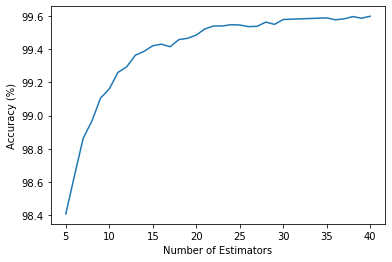
We have trained a Random forest classifier, which fits a number of decision tree estimators on the dataset and uses averaging to improve the predictive accuracy and reduce over-fitting. Test accuracy vs. number of estimators has been evaluated and it saturates after 35 (shown in the following figure). The optimal number of estimators has been taken from the tail end and set to be 40 for the analysis that follows.
We have evaluated the accuracy of the RF classifier on our test dataset. In the following, we report relevant ML metrics evaluation for RF, which we will later extend to the other classification algorithms.
| Scoring Metric | Performance Value |
|---|---|
| accuracy | 99.60% |
| balanced_accuracy_score | 96.52% |
| precision_score_macro | 0.9963 |
| recall_score_macro | 0.99951 |
| f1_score_macro | 0.9957 |
We also report the confusion matrix for this classifier:

As shown above, RF classifier shows one of the highest accuracies among all the ML methods considered in this study, which can be attributed to its ensembling method, resulting in better generalization.
6.2.6 MLP
Through manual tuning of hyperparameters, the architecture of MLP has been chosen which achieves reasonable test accuracy without having two complex an architecture. The input layer for this MLP consists of the 44 features from the raw sensor data we mentioned in the above. The MLP architecture in the study contains 3 fully connected layers of 100 neurons each with ReLU activation followed by Batch Normalization. L2 regularization has been adopted to thwart overfitting and aid generalization. A mini batch size of 256 samples, and a learning rate of 0.0001 have been chosen. For optimization, Adam optimizer has been chosen. The resulting architecture is shown in the following:

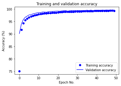
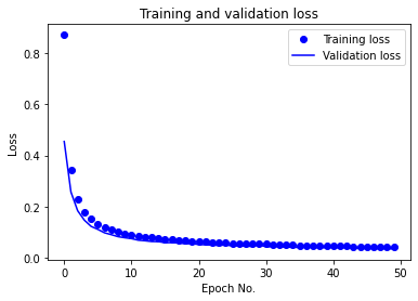
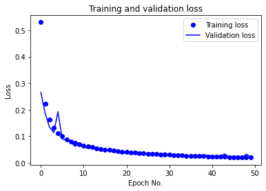
After running for 50 epochs, the aforementioned MLP achieves 99.56% test accuracy on raw data. The training/validation accuracy vs. epoch as well as training/validation loss vs. epoch plots are given below:

We also report the following evaluated ML metrics:
| Scoring Metric | Performance Value |
|---|---|
| accuracy | 99.56% |
| balanced_accuracy_score | 99.57% |
| precision_score_macro | 0.9952 |
| recall_score_macro | 0.9957 |
| f1_score_macro | 0.9955 |
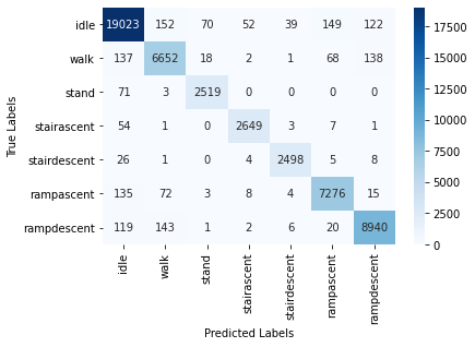
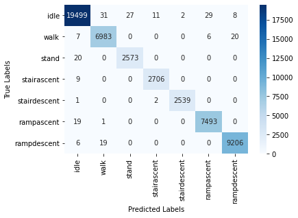
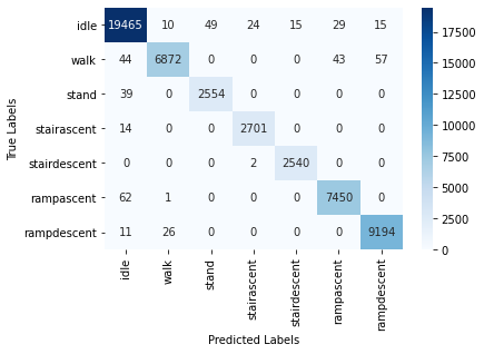
The high test accuracy is reflected in the Confusion Matrix plot as well:

PCA-MLP (where features have been projected into their principal subspaces) achieves 99.57% test accuracy with dimensionality reduction (keeping 30 PCA components,as lower number of components reduced test accuracy) and the same MLP architecture and training options, which is similar to training on just the raw data. The training/validation accuracy vs. epoch as well as training/validation loss vs. epoch plots for PCA-MLP are given below:

We also report the following evaluated ML metrics:
| Scoring Metric | Performance Value |
|---|---|
| accuracy | 99.57% |
| balanced_accuracy_score | 99.60% |
| precision_score_macro | 0.9951 |
| recall_score_macro | 0.9960 |
| f1_score_macro | 0.9956 |
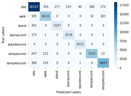
The high test accuracy is reflected in the Confusion Matrix plot as well:
Running for a higher number of epochs would translate to higher accuracy, and thorough hyper-parameter tuning is yet to be done, but the result is already quite good.
6.2.7 CNN
The CNN used in this study was configured with 3 convolutional layers and 1 fully connected layer. As our data is 1-dimensional, we employ a 1D-CNN on the data. The architecture chosen is shown in the following:

The hyper-parameters were tuned using manual search.
The learning rate was changed from the default of 0.001 due to severe oscillations in the validation accuracy and loss (as can be noticed from the following figure) throughout training. A value of 0.0001 yielded results with minimal oscillations in the validation accuracy and loss in the later epochs and overall smoother learning curves.
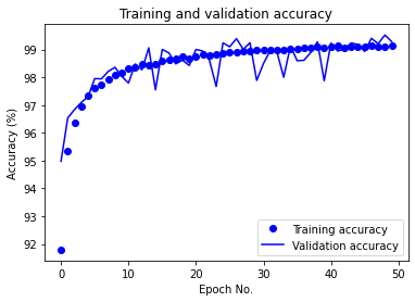
The number of epochs was initially chosen to be 100. It was reduced to 50 due to excessive learning time. Given the current results with the new learning rate, the model appears to converge at approximately 35 epochs, though further tuning could likely cause learning performance changes that could make 50 epochs or more necessary for convergence.
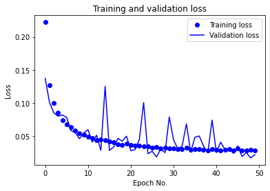
The CNN with the current configuration achieved a test accuracy of 99.14% on the raw data. In the following, we provide the training/validation accuracy vs. epoch as well as training/validation loss vs. epoch plots for CNN in the following:
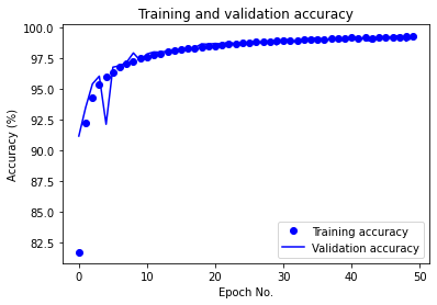
After performing evauation using ML metrics, for the partitioned training and testing dataset, we report the following performances:
| Scoring Metric | Performance Value |
|---|---|
| accuracy | 99.14% |
| balanced_accuracy_score | 99.12% |
| precision_score_macro | 0.9906 |
| recall_score_macro | 0.9912 |
| f1_score_macro | 0.9909 |
The high test accuracy is reflected in the Confusion Matrix plot as well:
The current results are good overall, and further tuning will be done to optimize the rest of the hyperparameters to improve learning and testing performance.
6.3 Comparative Analysis
In the following, we present a comparison among the test accuracies obtained from different methods studied so far:
| Method | Test Accuracy (%) |
|---|---|
| GaussianNB | 64.92 |
| LDA | 68.41 |
| DT | 96.75 |
| SVM | 93.81 |
| RF | 99.60 |
| PCA-LDA | 68.41 |
| MLP | 99.56 |
| PCA-MLP | 99.57 |
| CNN | 99.14 |
7 Conclusions and Future Directions
In this project, we have evaluated several unsupervised and supervised machine learning algorithms on raw data, and have obtained reasonable classification accuracy on test data for most of the methods. We have mostly worked on raw data, and from the results that we have, it appears that Goniometer sensors are the most informative, due to high SNR of the data. But with proper signal conditioning (such as windowed moving average), we expect that the other sensor data will become important predictors as well. From the accuracy metric, we can see that RF, MLP and PCA-MLP achieve the highest test accuracies, while CNN and DT achieve reasonably good accuracies. In this study, we focused on subject specific locomotion mode classification and we think that subject-agnostic classification can be an exiciting future direction.
8 Broader Impact
The broader impact of this project would be future development of robotic assistive devices and active prostheses for targeted rehabilitation methods beyond clinical settings, and improvement of biomimetic controllers that better adapt to terrain conditions (practical scenarios). Classification of locomotion modes from instantaneous samples with fast and effective inference may help in developing assistive devices with higher predictive capabilities.
9 Contributions
-
Ian Thomas Cullen: Data Cleaning, Data Pre-processing (Signal Conditioning using Windowed Moving Average), Feature Engineering (calculating max/min, mean, standard deviation etc. from raw features), Video Editing and Presentation for Proposal -
Kennedy A Lee: Convolutional Neural Network (CNN) on raw data, Hyperparameter Tuning -
Imran Ali Shah: Principal Component Analysis (PCA), k-Means Clustering, Naive Bayes (NB), Video Editing and Presentation for Proposal -
Anupam Golder: Data Merging, MRMR Feature Scoring, LDA, DT, SVM, RF, MLP/PCA-MLP, Github Page Editing
10 References
- Camargo, J., Ramanathan, A., Flanagan, W., & Young, A. (2021). A comprehensive, open-source dataset of lower limb biomechanics in multiple conditions of stairs, ramps, and level-ground ambulation and transitions. Journal of Biomechanics, 119, 110320.
- Kang, I., Molinaro, D. D., Duggal, S., Chen, Y., Kunapuli, P., & Young, A. J. (2021). Real-Time Gait Phase Estimation for Robotic Hip Exoskeleton Control During Multimodal Locomotion. IEEE Robotics and Automation Letters, 6(2), 3491-3497.
- Lee, D., Kang, I., Molinaro, D. D., Yu, A., & Young, A. J. (2021). Real-Time User-Independent Slope Prediction Using Deep Learning for Modulation of Robotic Knee Exoskeleton Assistance. IEEE Robotics and Automation Letters, 6(2), 3995-4000.
- Spiewak, C. (2018). A Comprehensive Study on EMG Feature Extraction and Classifiers. Open Access Journal of Biomedical Engineering and Biosciences, 1(1).
- Loh, W. Y., & Shih, Y. S. (1997). Split selection methods for classification trees. Statistica sinica, 815-840.
- Ding, C., & Peng, H. (2005). Minimum redundancy feature selection from microarray gene expression data. Journal of bioinformatics and computational biology, 3(02), 185-205.